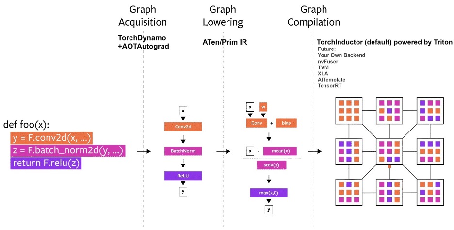
Graph acquisition in PyTorch refers to the process of creating and managing the computational graph that represents a neural network’s operations. This graph is central to PyTorch’s dynamic nature, allowing for flexible model architectures and efficient gradient computation. With the advent of tools like TorchScript, PyTorch Dynamo, and AOT Autograd, PyTorch continues to improve the performance and deployability of models without sacrificing its user-friendly interface. Understanding how PyTorch handles computational graphs is key to leveraging the full power of the framework.

PyTorch Dynamo TorchDynamo (torch._dynamo) is an internal API that uses a CPython feature called the Frame Evaluation API to safely capture PyTorch graphs. Methods that are available externally for PyTorch users are surfaced through the torch.compiler namespace.

Benefits of PyTorch Dynamo Performance Gains: By optimizing the execution graph on the fly, Dynamo can significantly speed up the performance of PyTorch models, particularly for models with a lot of small operations that can be fused together. Ease of Use: Dynamo does not require any changes to the existing PyTorch code, making it very easy to adopt. Flexibility: Since Dynamo operates dynamically, it can handle the dynamic computation graphs that are typical in PyTorch, including graphs with loops and conditionals.

Example Model (Simple 2 Layer NN)

1
2
3
4
5
6
7
8
9
10
11
12
# Define your PyTorch model
class MyModel(nn.Module):
    def __init__(self):
        super(MyModel, self).__init__()
        self.fc1 = nn.Linear(10, 5)
        self.fc2 = nn.Linear(5, 2)
        self.relu= nn.ReLU()
        self.softmax=nn.Softmax(dim=1)
    
    def forward(self, x):
        result = self.softmax(self.fc2(self.relu(self.fc1(x))))
        return result

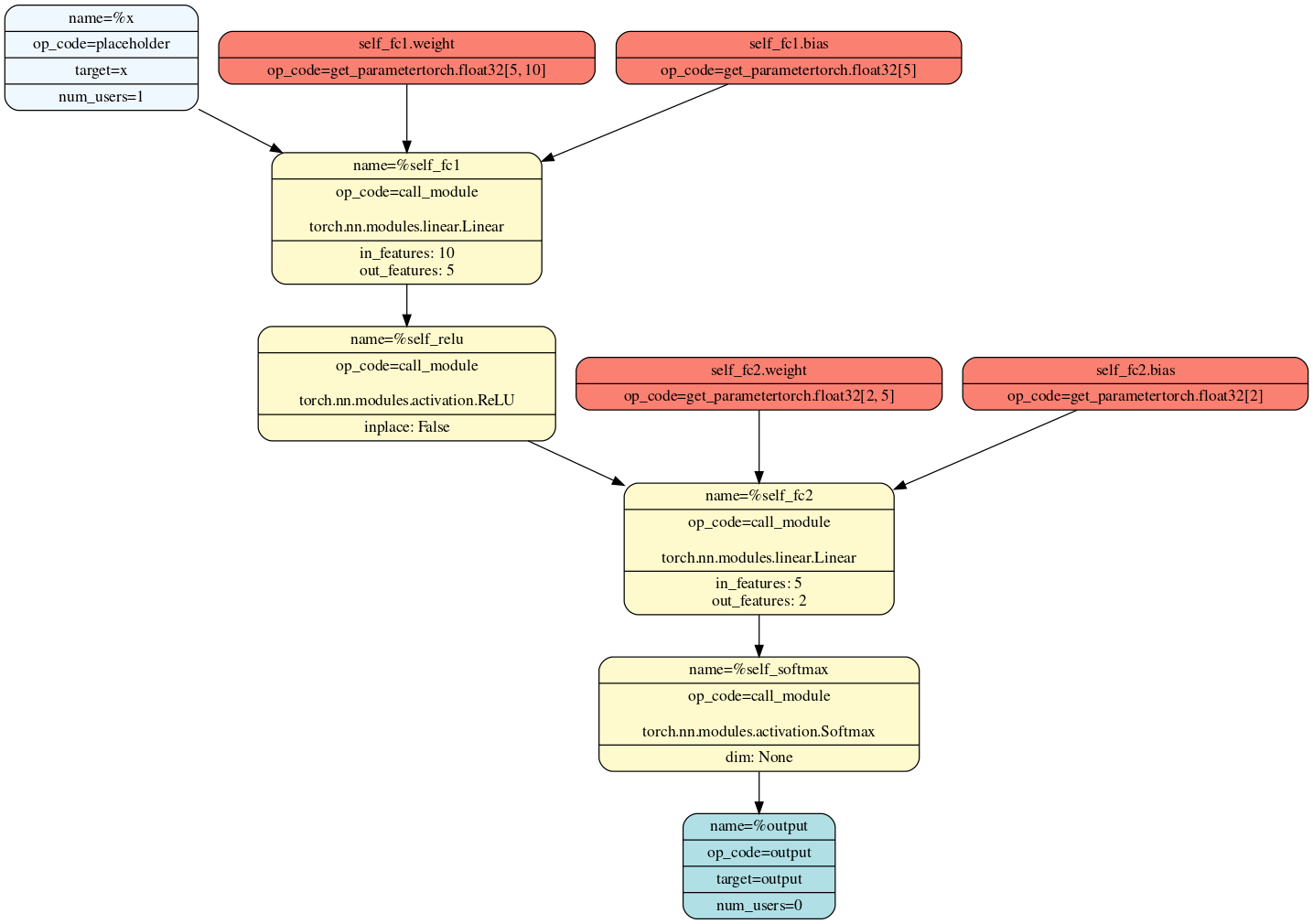
The model defined in the code snippet is a simple feedforward neural network implemented using PyTorch’s nn.Module. It consists of two fully connected layers (nn.Linear) with a ReLU activation function (nn.ReLU) applied after the first layer and a softmax activation function (nn.Softmax) applied after the second layer.

Create Forward Graph with Torch Dynamo

Code Snippet for Dynamo Backend for Saving Graph to SVG:

1
2
3
4
5
6
def dynamo_backend(gm, sample_inputs):
    code = gm.print_readable()
    gm.graph.print_tabular()
    with open("model_graph.svg", "wb") as file:
        file.write(FxGraphDrawer(gm,'f').get_dot_graph().create_svg())
    return gm.forward

Compile the model and perform forward pass:

1
2
3
4
5
6
7
8
model = MyModel()
input_tensor = torch.randn(1, 10)
torch._dynamo.reset()
# Compile the model with Dynamo
compiled_f = torch.compile(model, backend=dynamo_backend)

# Forward Pass
out = compiled_f(input_tensor)

This is the generated graph for forward pass:

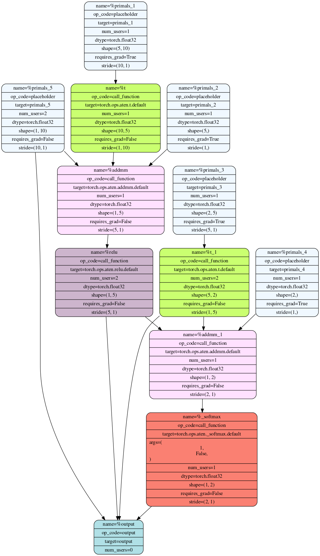
AOTAutograd

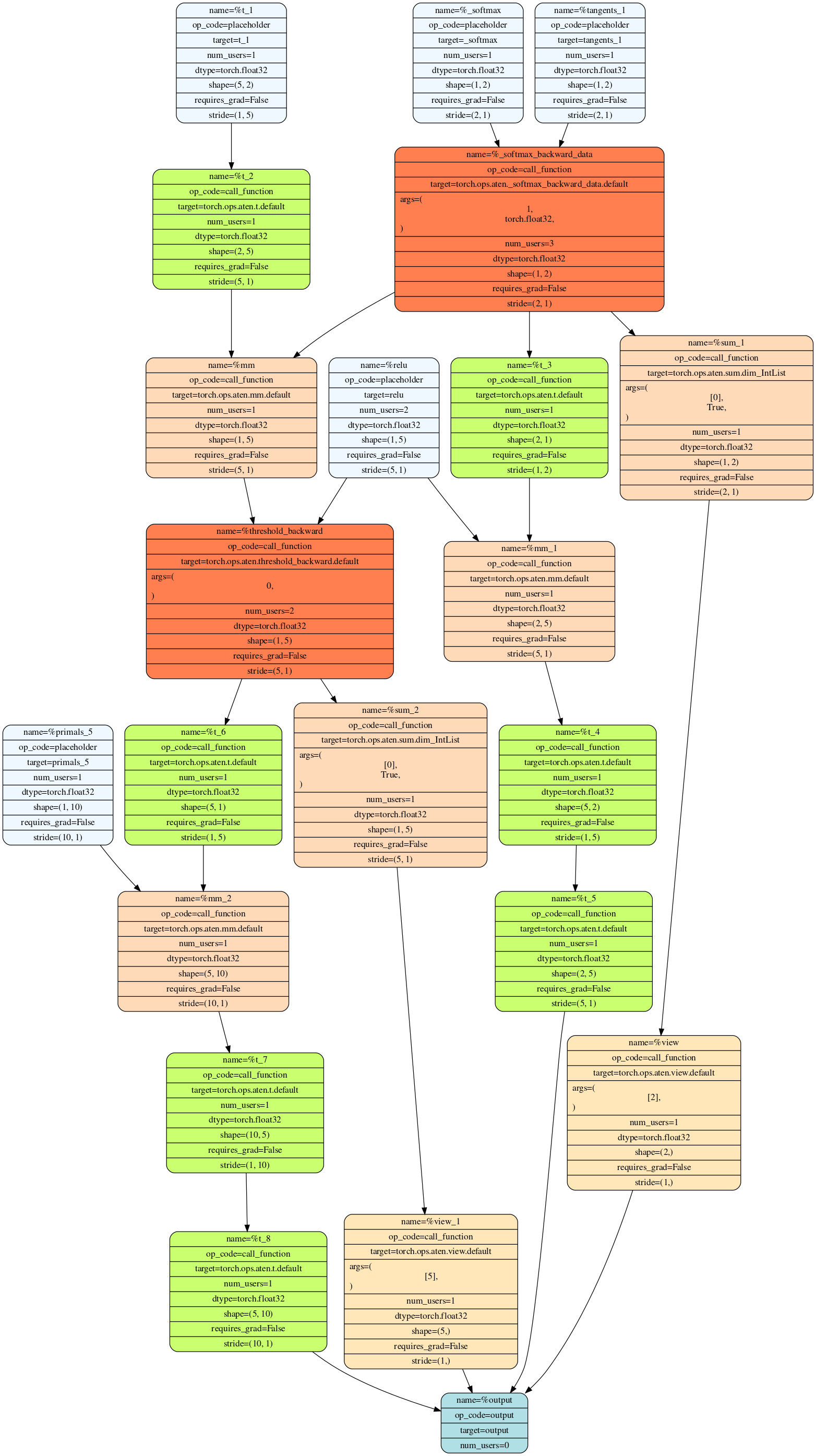
AOTAutograd captures not only the user-level code, but also backpropagation, which results in capturing the backwards pass “ahead-of-time”. This enables acceleration of both forwards and backwards pass using TorchInductor.

Benefits of AOTAutograd

AOT Autograd works by analyzing the forward pass of your model and generating an optimized backward pass ahead of time. This is in contrast to the traditional approach where the backward pass is dynamically generated during runtime. By doing this ahead of time, AOT Autograd can apply optimizations that are not possible at runtime.

• Training Speed: AOT Autograd can reduce the overhead of the backward pass, leading to faster training times.
• Customization: It allows for customization of the backward pass, enabling more control over the training process.
• Integration: AOT Autograd is designed to work seamlessly with existing PyTorch models, making it easy to integrate into current workflows.

Create Forward & Backward Graph with AOT Autograd

Code Snippet for AOT Backend for Saving Graph to SVG:

1
2
3
4
5
6
7
8
9
10
11
12
13
14
15
16
17
18
19
20
21
22
23
def aot_backend(gm, sample_inputs): 
    # Forward compiler capture
    def fw(gm, sample_inputs):
        gm.print_readable()
        g = FxGraphDrawer(gm, 'fn')
        with open("forward_aot.svg", "wb") as file:
            file.write(g.get_dot_graph().create_svg())
        return make_boxed_func(gm.forward)
    
    # Backward compiler capture
    def bw(gm, sample_inputs):
        gm.print_readable()
        g = FxGraphDrawer(gm, 'fn')
        with open("backward_aot.svg", "wb") as file:
            file.write(g.get_dot_graph().create_svg())
        return make_boxed_func(gm.forward)
    
    # Call AOTAutograd
    gm_forward = aot_module_simplified(gm,sample_inputs,
                                       fw_compiler=fw,
                                       bw_compiler=bw)

    return gm_forward

Compile the model and perform forward and backward pass:

1
2
3
4
5
6
7
8
9
10
11
12
13
14
15
model = MyModel()

input_tensor = torch.randn(1, 10)
ouput = torch.randn(2)

torch._dynamo.reset()

# Compile the model with AOT Backend
compiled_f = torch.compile(model, backend=aot_backend)

# Calculate Loss from Forward Pass
loss= torch.nn.functional.mse_loss(compiled_f(input_tensor), ouput)

# Perform Backward Pass
out = loss.backward()

These are the generated graphs for forward and backward pass:

Conclusion

PyTorch Dynamo and AOT Autograd are exciting developments for the PyTorch community. They offer the potential for significant performance improvements while maintaining the flexibility and ease of use that PyTorch users have come to appreciate. As these features continue to mature, they will likely become integral parts of the PyTorch ecosystem, helping to bridge the gap between rapid prototyping and efficient production deployment.

Both PyTorch Dynamo and AOT Autograd are tools aimed at improving the performance of PyTorch models by optimizing the execution of operations. While Dynamo focuses on runtime optimizations, AOT Autograd looks at optimizing the backward pass ahead of time. These tools can be particularly useful when you’re looking to scale up your models and need to squeeze out extra performance without significant refactoring of your existing codebase.