Quantization transforms floating-point values (‘float32’) into lower-precision formats, such as 8-bit integers (‘int8’), while attempting to preserve the numerical range and accuracy of the original data. This reduces memory usage and computation time.
In PyTorch, quantization can be implemented at various stages:
- Static Quantization: Applied after training using calibration.
- Dynamic Quantization: Quantization parameters are computed during inference.
- Quantization-Aware Training (QAT): Simulates quantization during training for higher accuracy.
1. Key Concepts in Quantization
Quantization Formula
Quantization maps a floating-point value ( x ) to an integer ( q ):
\[q = \text{round}\left(\frac{x}{\text{scale}} + \text{zeropoint}\right)\]-
Scale: Represents the step size or resolution of the quantized values. It defines how large a step in the integer domain corresponds to a change in the floating-point domain. The scale is derived from the range of the floating-point values divided by the range of the quantized integers.
-
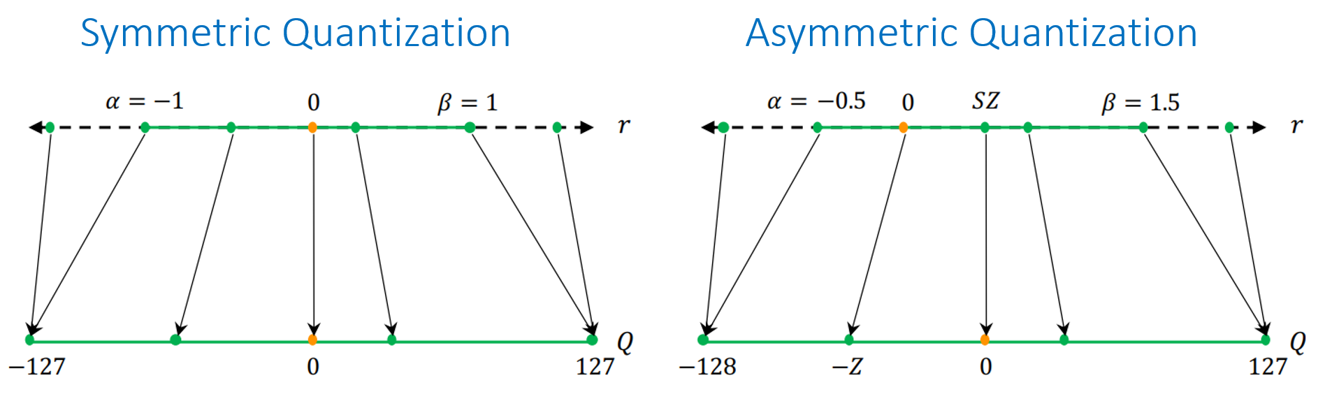
Zero Point: A value in the integer range that corresponds to the floating-point zero. It ensures that quantization accurately maps zero from the floating-point domain to the integer domain, minimizing errors when zero plays a critical role in computations. The zero point ensures that the quantized range properly represents the dynamic range of the original floating-point numbers, especially when the range doesn’t start at zero (asymmentric quantization). It acts as an offset, allowing negative or positive floating-point values to be correctly mapped into the integer domain.
Dequantization Formula
To recover the original value:
\[\hat{x} = \text{scale} \cdot (q - \text{zeropoint})\]Dequantization is typically performed after computations to interpret quantized results.
2. Example Tensor for Quantization Per Tensor and Quantization Per Channel
Given weights tensor (2 channels):
\[\text{Weights} = \begin{bmatrix} 1.0 & 2.0 & 3.0 \\ 4.0 & 5.0 & 6.0 \end{bmatrix}\]Shape: ([2, 3])
Integer range: ([-128, 127])
2.1 Per-Tensor Quantization
We will quantize a tensor of weights into an 8-bit integer range ([128,127]). This method works well for tensors where the values across all channels share a similar dynamic range. However, if each channel has distinct ranges, this approach may lead to significant quantization errors.
- Global Min/Max: The minimum and maximum values across the entire tensor are computed. These values define the dynamic range for quantization.
- Scale and Zero Point: The scale represents the step size for quantization, and the zero point determines the integer value corresponding to the minimum floating-point value. The formulas for computing scale and zero point ensure that the mapping is linear and reversible.
- Quantization: Each floating-point value is converted to an integer using the quantization formula, maintaining the relative spacing between values.
- Dequantization: The integers are mapped back to floating-point values using the inverse of the quantization formula.
Step 1: Compute Global Min/Max
- Global Min: = 1.0
- Global Max: = 6.0
Step 2: Compute Scale and Zero Point
The scale is calculated as:
\[\text{scale} = \frac{x_{\text{max}} - x_{\text{min}}}{q_{\text{max}} - q_{\text{min}}} = \frac{6.0 - 1.0}{255} = 0.01961\]The scale of 0.01961 means each step in the quantized integer domain corresponds to an increment of 0.01961 in the floating-point domain.
\[\text{zeropoint} = \text{round}(-128 - \frac{x_{\text{min}}}{\text{scale}}) = \text{round}(-128 - \frac{1.0}{0.01961}) = \text{round}(-179.99) = -180\]The zero point of −180 ensures that 0.0 in the floating-point domain maps to an integer value of −180.
Step 3: Quantize
Apply the quantization formula:
\[q = \text{round}\left(\frac{x}{\text{scale}} + \text{zeropoint}\right)\]Quantized values:
\[\begin{align} q(1.0) = \text{round}\left(\frac{1.0}{0.01961} - 180\right) = \text{round}(0) = 0 \\ \\ q(2.0) = \text{round}\left(\frac{2.0}{0.01961} - 180\right) = \text{round}(51.02) = 51 \\ \\ q(3.0) = \text{round}\left(\frac{3.0}{0.01961} - 180\right) = \text{round}(102.04) = 102 \\ \\ q(4.0) = \text{round}\left(\frac{4.0}{0.01961} - 180\right) = \text{round}(153.06) = 153 \\ \\ q(5.0) = \text{round}\left(\frac{5.0}{0.01961} - 180\right) = \text{round}(204.08) = 204 \\ \\ q(6.0) = \text{round}\left(\frac{6.0}{0.01961} - 180\right) = \text{round}(255.0) = 255 \end{align}\]So this transformed floating-point values (‘float32’) into lower-precision formats 8-bit integers (‘int8’)
\[\text{Weights} = \begin{bmatrix} 0 & 51 & 102 \\ 153 & 204 & 255 \end{bmatrix}\]Step 4: Dequantize
Dequantization reverses this process, converting the integer values back to floating-point approximations. Together, quantization and dequantization enable efficient computations without significantly compromising model accuracy.
\[\hat{x} = \text{scale} \cdot (q - \text{zeropoint})\]Dequantized values:
\[\begin{align} \hat{x}(0) = 0.01961 \cdot (0 - (-180)) = 1.0 \\ \\ \hat{x}(51) = 0.01961 \cdot (51 - (-180)) = 2.0 \\ \\ \hat{x}(102) = 0.01961 \cdot (102 - (-180)) = 3.0 \\ \\ \hat{x}(153) = 0.01961 \cdot (153 - (-180)) = 4.0 \\ \\ \hat{x}(204) = 0.01961 \cdot (204 - (-180)) = 5.0 \\ \\ \hat{x}(255) = 0.01961 \cdot (255 - (-180)) = 6.0 \end{align}\]Quantization Error
Quantization error is the difference between the original floating-point value and its quantized approximation. It arises because a finite set of integers cannot perfectly represent an infinite set of floating-point numbers.
Quantization error is:
\[\text{Error} = x - \hat{x}\]For per-tensor quantization in this case, the error is 0 for all values, as the range is perfectly covered.
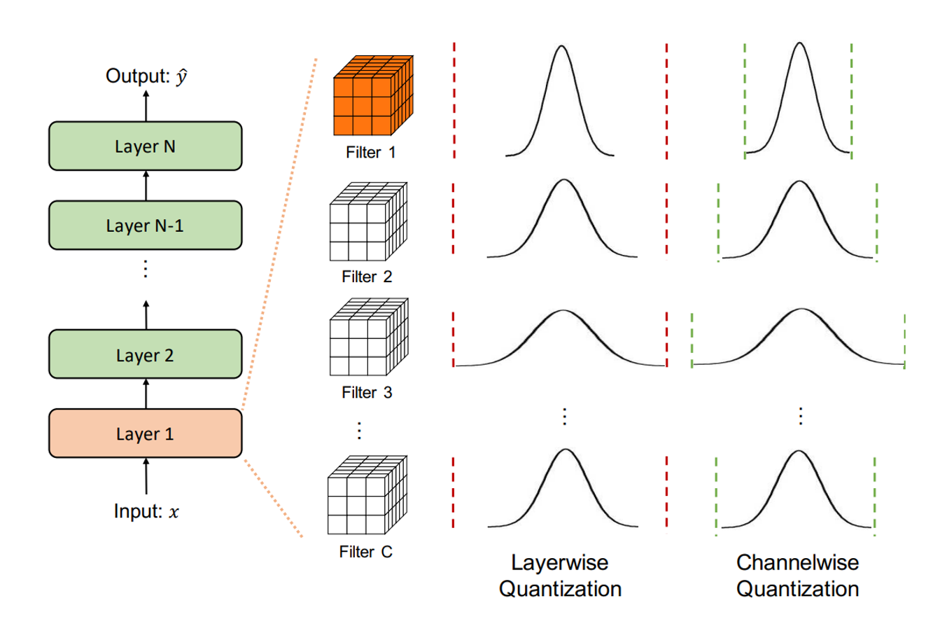
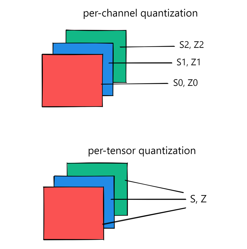
2.2 Per-Channel Quantization
Per-channel quantization is a quantization technique where each channel of a tensor (e.g., in a convolutional layer) is quantized using its own unique scale and zero point, rather than applying a single shared scale and zero point across the entire tensor (as in per-tensor quantization).
- Channel-Wise Min/Max: The minimum and maximum values are computed separately for each channel.
- Channel-Wise Scale and Zero Point: Each channel gets its own scale and zero point, allowing better handling of varying dynamic ranges.
- Quantization and Dequantization: Each channel is quantized and dequantized using its respective scale and zero point.
- Error: The quantization error is also 0 in this case, as the independent channel-wise computation ensures accurate mapping.
Step 1: Compute Min/Max for Each Channel
- Channel 1: ([1.0, 2.0, 3.0]), Min = (1.0), Max = (3.0)
- Channel 2: ([4.0, 5.0, 6.0]), Min = (4.0), Max = (6.0)
Step 2: Compute Scale and Zero Point for Each Channel
Channel 1:
\[\text{scale}_1 = \frac{3.0 - 1.0}{255} = 0.007843\] \[\text{zeropoint}_1 = \text{round}(-128 - \frac{1.0}{0.007843}) = \text{round}(-128 - 127.5) = -255\]Channel 2:
\[\text{scale}_2 = \frac{6.0 - 4.0}{255} = 0.007843\] \[\text{zeropoint}_2 = \text{round}(-128 - \frac{4.0}{0.007843}) = \text{round}(-128 - 510) = -638\]Step 3: Quantize and Dequantize
Channel 1 Quantized Values:
\[\begin{align} q(1.0) = \text{round}\left(\frac{1.0}{0.007843} + 255\right) = 127 \\ \\ q(2.0) = \text{round}\left(\frac{2.0}{0.007843} + 255\right) = 255 \\ \\ q(3.0) = \text{round}\left(\frac{3.0}{0.007843} + 255\right) = 383 \end{align}\]Channel 1 Dequantized Values:
\[\begin{align} \hat{x}(127) = 0.007843 \cdot (127 - 255) = 1.0 \\ \\ \hat{x}(255) = 0.007843 \cdot (255 - 255) = 2.0 \\ \\ \hat{x}(383) = 0.007843 \cdot (383 - 255) = 3.0 \end{align}\]Channel 2 Quantized Values:
\[\begin{align} q(4.0) = \text{round}\left(\frac{4.0}{0.007843} + 638\right) = 510 \\ \\ q(5.0) = \text{round}\left(\frac{5.0}{0.007843} + 638\right) = 766 \\ \\ q(6.0) = \text{round}\left(\frac{6.0}{0.007843} + 638\right) = 1022 \end{align}\]Channel 2 Dequantized Values:
\[\begin{align} \hat{x}(510) = 0.007843 \cdot (510 - 638) = 4.0 \\ \\ \hat{x}(766) = 0.007843 \cdot (766 - 638) = 5.0 \\ \\ \hat{x}(1022) = 0.007843 \cdot (1022 - 638) = 6.0 \end{align}\]Quantization Error
Quantization error is the difference between the original floating-point value and its quantized approximation. It arises because a finite set of integers cannot perfectly represent an infinite set of floating-point numbers.
In this case, the error is 0 for all values, as the quantization was exact for each channel.
3. Code Snippet For Custom Quant and Dequant
1
2
3
4
5
6
7
8
9
10
11
12
13
14
15
16
17
18
19
20
21
22
23
24
25
26
27
28
29
30
31
32
33
34
35
36
37
38
39
40
41
42
43
44
45
46
47
48
49
50
51
52
53
54
55
56
57
58
59
60
61
62
63
64
65
66
67
68
69
70
71
72
73
import torch

# Tensor values
weights = torch.tensor([
    [1.0, 2.0, 3.0],
    [4.0, 5.0, 6.0]
])

# Quantization parameters for per-tensor quantization
qmin, qmax = -128, 127
x_min, x_max = weights.min().item(), weights.max().item()

# Per-tensor scale and zero-point
scale_tensor = (x_max - x_min) / (qmax - qmin)
zeropoint_tensor = round(-x_min / scale_tensor)

# Per-channel quantization parameters
x_min_channel = weights.min(dim=1).values
x_max_channel = weights.max(dim=1).values
scale_channel = (x_max_channel - x_min_channel) / (qmax - qmin)
zeropoint_channel = torch.round(-x_min_channel / scale_channel)


def quant(x, scale, zeropoint):
    """
    Quantize the input tensor.
    Args:
        x (torch.Tensor): The input tensor to quantize.
        scale (float or torch.Tensor): The quantization scale.
        zeropoint (float or torch.Tensor): The quantization zero-point.
    Returns:
        torch.Tensor: Quantized tensor.
    """
    q = torch.round(x / scale + zeropoint)
    q = torch.clamp(q, qmin, qmax)  # Clamp to quantized range
    return q.int()


def dequant(q, scale, zeropoint):
    """
    Dequantize the quantized tensor.
    Args:
        q (torch.Tensor): The quantized tensor.
        scale (float or torch.Tensor): The quantization scale.
        zeropoint (float or torch.Tensor): The quantization zero-point.
    Returns:
        torch.Tensor: Dequantized tensor.
    """
    return scale * (q - zeropoint)


# Per-tensor quantization
q_tensor = quant(weights, scale_tensor, zeropoint_tensor)
dq_tensor = dequant(q_tensor, scale_tensor, zeropoint_tensor)

# Per-channel quantization
q_channel = quant(weights, scale_channel.view(-1, 1), zeropoint_channel.view(-1, 1))
dq_channel = dequant(q_channel, scale_channel.view(-1, 1), zeropoint_channel.view(-1, 1))

# Output results
print("Original Weights:")
print(weights)

print("\nPer-Tensor Quantized Weights:")
print(q_tensor)
print("\nPer-Tensor Dequantized Weights:")
print(dq_tensor)

print("\nPer-Channel Quantized Weights:")
print(q_channel)
print("\nPer-Channel Dequantized Weights:")
print(dq_channel)
Comparison
| Metric | Per-Tensor | Per-Channel |
|---|---|---|
| Scale | 0.01961 | [0.007843, 0.007843] |
| Zero Point | -180 | [-255, -638] |
| Quantization Error | 0 | 0 |
Although this example has error zero for both but if you try another shapes, you can see that per-channel quantization is more suitable for handling varying dynamic ranges across channels, reducing quantization errors significantly in practical scenarios.
4. Quantization Types
a. Static Quantization
- Weights and activations are quantized.
- Involves precomputing scale and zero-point values during calibration.
- Best for use cases with predictable inputs and stable computational patterns.
Example in PyTorch:
1
2
3
4
5
6
7
8
9
10
11
12
13
14
15
16
17
18
19
20
import torch
import torch.quantization as quant

# Define a model
model = torch.nn.Sequential(
    torch.nn.Linear(4, 2),
    torch.nn.ReLU()
)

# Prepare for static quantization
model.qconfig = quant.get_default_qconfig('fbgemm')
prepared_model = quant.prepare(model)

# Calibrate with representative data
data = torch.randn(100, 4)
for sample in data:
    prepared_model(sample)

# Convert to quantized model
quantized_model = quant.convert(prepared_model)
b. Dynamic Quantization
- Only weights are quantized; activations remain in floating-point.
- Ideal for models dominated by linear layers, like transformers and RNNs.
Example in PyTorch:
1
2
3
4
5
6
7
8
9
import torch

# Define a model
model = torch.nn.Linear(4, 2)

# Apply dynamic quantization
quantized_model = torch.quantization.quantize_dynamic(
    model, {torch.nn.Linear}, dtype=torch.qint8
)
c. Quantization-Aware Training (QAT)
- Simulates quantized inference during training.
- Results in higher accuracy than static or dynamic quantization.
Example in PyTorch:
1
2
3
4
5
6
7
8
9
10
11
12
13
14
15
16
17
18
19
20
21
22
23
24
import torch
import torch.quantization as quant

# Define a model
model = torch.nn.Sequential(
    torch.nn.Linear(4, 2),
    torch.nn.ReLU()
)

# Prepare for QAT
model.qconfig = quant.get_default_qat_qconfig('fbgemm')
prepared_model = quant.prepare_qat(model)

# Train the model
optimizer = torch.optim.SGD(prepared_model.parameters(), lr=0.01)
for epoch in range(10):
    optimizer.zero_grad()
    output = prepared_model(torch.randn(10, 4))
    loss = output.mean()
    loss.backward()
    optimizer.step()

# Convert to quantized model
quantized_model = quant.convert(prepared_model)
5. Practical Considerations
- Calibration Data: The representativeness of calibration data directly impacts quantization accuracy.
- Hardware Support: Quantized models must be deployed on hardware that supports integer arithmetic (e.g., ARM, NVIDIA, Intel).
- Accuracy vs. Efficiency: Quantization may lead to accuracy loss. Techniques like QAT can mitigate this.
Conclusion
Quantization and dequantization are vital tools for making machine learning models efficient and deployable on resource-constrained devices. By understanding and implementing these techniques in PyTorch, you can leverage their power to optimize models for real-world applications while maintaining acceptable accuracy.