When dealing with symmetric and positive-definite matrices, Cholesky decomposition emerges as an indispensable tool in numerical computing. This matrix factorization technique not only simplifies complex computations but also finds applications in a wide array of real-world problems.

What is Cholesky Decomposition?

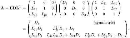
Cholesky decomposition is a method to factor a symmetric positive-definite matrix ( A ) into the product of a lower triangular matrix ( L ) and its transpose ( L^T ), as shown:

If ( A ) is a complex matrix, the transpose ( L^T ) is replaced by the conjugate transpose ( L^H ).

This factorization is only possible when ( A ) is symmetric and positive-definite:

• Symmetric: ( A = A^T ), meaning the matrix is equal to its transpose.
• Positive-definite: All eigenvalues of ( A ) are positive, which ensures that ( A ) has no zero or negative values along its diagonal.

Cholesky decomposition is unique, which makes it particularly useful for a variety of numerical methods. Let’s explore its mathematical intuition before diving into its use cases.

Mathematical Intuition Behind Cholesky Decomposition

The intuition behind Cholesky decomposition is that it simplifies working with symmetric matrices by breaking them down into simpler, triangular matrices. The core idea is:

• A symmetric positive-definite matrix ( A ) can be thought of as representing a quadratic form, i.e., a scalar function of vector inputs: \(x^T A x\) where ( x ) is a vector.

• Cholesky decomposition provides an efficient way to rewrite this quadratic form in terms of a simpler triangular matrix ( L ), which reduces complexity when solving linear systems.

Matrix Decomposition

Consider the matrix ( A ). Instead of performing direct matrix operations on ( A ), the Cholesky decomposition transforms ( A ) into a simpler triangular matrix ( L ), such that:

This decomposition provides several computational benefits, such as reducing the time complexity of matrix operations from ( O(n^3) ) to ( O(n^2) ). This speedup makes Cholesky decomposition attractive in algorithms where performance is critical, such as optimization or solving linear equations.

Use Cases of Cholesky Decomposition

Cholesky decomposition is widely used in several real-world applications, particularly in areas that require solving linear systems or working with large symmetric matrices. Let’s explore some of its most common use cases:

1. Solving Linear Systems

One of the most practical uses of Cholesky decomposition is solving systems of linear equations of the form:

Where ( A ) is a symmetric positive-definite matrix, and ( b ) is a vector of constants. Instead of directly solving this equation, we can use Cholesky decomposition to reduce the computational complexity. The steps are:

1. Decompose:
   \(A = L \cdot L^T\)

2. Solve this equation:
   \(L y = b\)

3. Then Solve this equation:
   \(L^T x = y\)

Since ( L ) is a triangular matrix, solving these equations is computationally efficient.

2. Optimization Algorithms

In optimization problems like nonlinear least squares, linear regression, or conjugate gradient methods, Cholesky decomposition helps minimize objective functions. Since optimization often involves inverting large positive-definite Hessian matrices, decomposing them with Cholesky leads to faster computations.

3. Monte Carlo Simulation

In Monte Carlo simulations, Cholesky decomposition is used to generate correlated random variables. The covariance matrix of these random variables is often positive-definite and symmetric. Using Cholesky decomposition on the covariance matrix allows generating samples that adhere to the desired correlation structure.

4. Kalman Filters

In control theory and signal processing, Kalman filters are used to estimate the state of a system over time. Since Kalman filters frequently rely on covariance matrices, which are symmetric and positive-definite, Cholesky decomposition is used for efficient matrix inversion and update steps in the filtering process.

Example: Performing Cholesky Decomposition with PyTorch

Let’s now walk through a simple example in PyTorch to see Cholesky decomposition in action.

Step 1: Create a Symmetric Positive-Definite Matrix

We begin by creating a random complex matrix and transforming it into a Hermitian positive-definite matrix.

1
2
3
4
5
6
7
8
9
import torch

# Step 1: Create a random 2x2 complex matrix
A = torch.randn(2, 2, dtype=torch.complex128)

# Create a Hermitian positive-definite matrix
A = A @ A.T.conj() + torch.eye(2, dtype=torch.complex128)
print("Original Hermitian Positive-Definite Matrix A:")
print(A)

Step 2: Apply Cholesky Decomposition

Next, we apply the Cholesky decomposition to factorize the matrix:

1
2
3
4
# Step 2: Perform Cholesky decomposition
L = torch.linalg.cholesky(A)
print("Lower Triangular Matrix L from Cholesky Decomposition:")
print(L)

Step 3: Verify the Decomposition

Finally, we verify that our decomposition was successful by reconstructing the matrix and checking if it matches the original:

1
2
3
4
5
6
7
8
# Step 3: Verify the decomposition
reconstructed_A = L @ L.T.conj()
print("Reconstructed Matrix from L:")
print(reconstructed_A)

# Check if the reconstruction is close to the original matrix
error = torch.dist(reconstructed_A, A)
print(f"Reconstruction Error: {error}")

If the decomposition is correct, the error should be close to zero.

Why Cholesky Decomposition is Efficient

The beauty of Cholesky decomposition lies in its computational efficiency. Let’s compare it to other common matrix factorizations:

• LU Decomposition: While LU decomposition works for a broader class of matrices, it has higher computational overhead for symmetric matrices.
• QR Decomposition: QR decomposition is also popular but requires more computations than Cholesky decomposition when dealing with positive-definite matrices.

Since Cholesky decomposition takes advantage of the symmetry and positive-definiteness of the matrix, it reduces the number of computations by about half compared to LU decomposition, making it preferable in many scenarios.

Conclusion

Cholesky decomposition is a powerful matrix factorization technique that simplifies working with symmetric positive-definite matrices. Its mathematical efficiency and wide applicability in solving linear systems, optimization problems, and probabilistic models make it a valuable tool in both theoretical and applied mathematics. By using libraries like PyTorch, you can easily leverage Cholesky decomposition in your own projects, ensuring faster and more accurate computations.

Next time you’re working with a symmetric positive-definite matrix, try Cholesky decomposition and enjoy the computational benefits it provides!