In the realm of deep learning, model performance is paramount. Whether you’re working on image classification, object detection, or any other computer vision task, the efficiency of your model can make or break your application. PyTorch Profiler is an invaluable tool for developers looking to optimize their models. It provides detailed insights into the time and memory consumption of model operations during execution. In this article, we’ll explore how to use PyTorch Profiler with a ResNet model to identify and address performance bottlenecks.

Setting Up the Environment: Before diving into profiling, ensure that PyTorch is installed in your environment. If not, you can easily install it using pip with the following command:

1
pip install torch torchvision

Once PyTorch is installed, you’re ready to start profiling your model.

Profiling a ResNet Model:

Step 1. Importing Necessary Modules Begin by importing the required modules from PyTorch and torchvision:

1
2
3
import torch
import torchvision.models as models
from torch.profiler import profile, record_function, ProfilerActivity

Step 2. Loading the Model Load a pre-trained ResNet model, such as ResNet-18, from the torchvision library:

1
model = models.resnet18(pretrained=True)

Step 3. Preparing the Input Create a dummy input tensor that simulates a batch of images with the appropriate dimensions for ResNet (3 color channels, 224x224 pixels):

1
input = torch.randn(1, 3, 224, 224)

Step 4. Setting Up the Device Determine if a GPU is available and move the model and input tensor to the GPU for faster computation:

1
2
3
device = torch.device("cuda" if torch.cuda.is_available() else "cpu")
model.to(device)
input = input.to(device)

Step 5. Switching to Evaluation Mode Ensure the model is in evaluation mode to disable training-specific behaviors:

1
model.eval()

Step 6. Profiling the Model Use the PyTorch Profiler within a context manager, specifying the activities to profile (CPU and CUDA) and enabling tensor shape recording:

1
2
3
with profile(activities=[ProfilerActivity.CPU, ProfilerActivity.CUDA], record_shapes=True) as prof:
    with record_function("model_inference"):
        model(input)

Step 7. Analyzing the Results After running the model inference, print the profiler output, focusing on the operations that consume the most CPU time:

1
print(prof.key_averages().table(sort_by="cpu_time_total", row_limit=10))

1
2
3
4
5
6
7
8
9
10
11
12
13
14
15
16
17
18
STAGE:2024-04-04 05:57:18 263803:263803 ActivityProfilerController.cpp:311] Completed Stage: Warm Up
STAGE:2024-04-04 05:57:21 263803:263803 ActivityProfilerController.cpp:317] Completed Stage: Collection
STAGE:2024-04-04 05:57:21 263803:263803 ActivityProfilerController.cpp:321] Completed Stage: Post Processing
----------------------------------  ------------  ------------  ------------  ------------  ------------  ------------  
                              Name    Self CPU %      Self CPU   CPU total %     CPU total  CPU time avg    # of Calls  
----------------------------------  ------------  ------------  ------------  ------------  ------------  ------------  
                   model_inference         0.11%       3.381ms       100.00%        3.072s        3.072s             1  
                      aten::conv2d         0.00%     107.000us        13.72%     421.551ms      21.078ms            20  
                 aten::convolution         0.01%     265.000us        13.72%     421.444ms      21.072ms            20  
                aten::_convolution         0.01%     181.000us        13.71%     421.179ms      21.059ms            20  
    aten::convolution_overrideable        13.69%     420.660ms        13.71%     420.998ms      21.050ms            20  
                       aten::empty         0.03%     834.000us         0.03%     834.000us       7.943us           105  
                        aten::add_         0.65%      20.077ms         0.65%      20.077ms     717.036us            28  
                  aten::batch_norm         0.00%      81.000us        83.99%        2.580s     128.997ms            20  
      aten::_batch_norm_impl_index         0.01%     193.000us        83.98%        2.580s     128.993ms            20  
           aten::native_batch_norm        83.96%        2.579s        83.98%        2.580s     128.981ms            20  
----------------------------------  ------------  ------------  ------------  ------------  ------------  ------------  
Self CPU time total: 3.072s

Step 8. Using tracing functionality

1
prof.export_chrome_trace("trace.json")

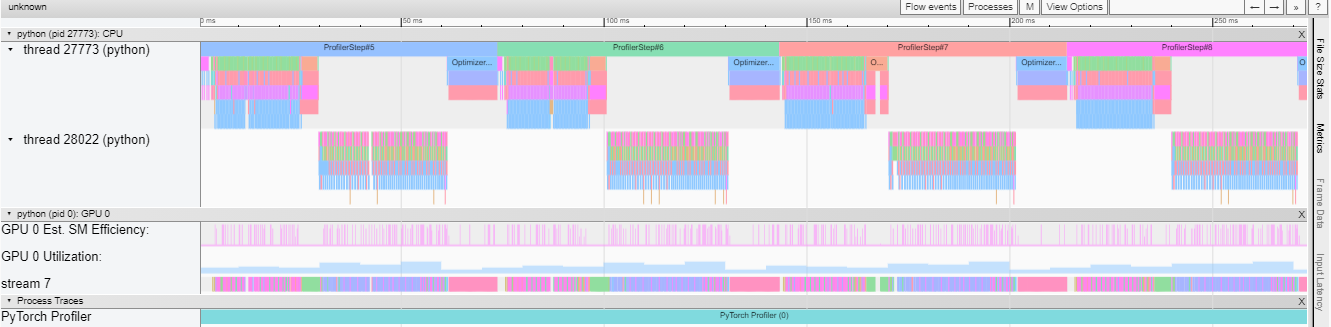
You can examine the sequence of profiled operators and CUDA kernels in Chrome trace viewer (chrome://tracing):

Chrome Tracer Viewer

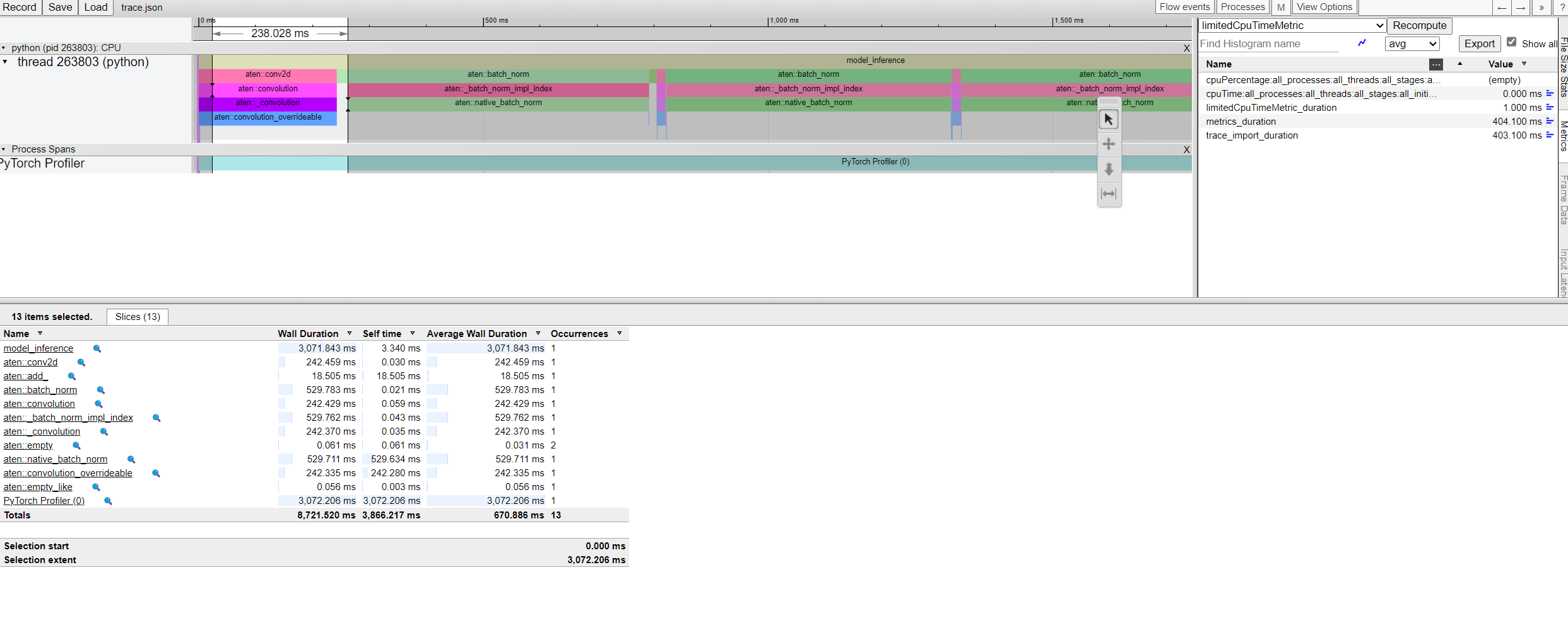
The profiler output will present a table summarizing the performance of various operations within the model. This table includes the time spent on each operation and the shapes of the tensors involved.